Have you ever wondered how a computer “learns” to recognize cats in pictures? Or do you want to guess the next word you will type? Fasten your seatbelts because we’re exploring the hidden power of neural networks, brain-inspired technology from the wonder of mathematics.
Let us understand the equations that dance with neurons, algorithms that apply learning, and magic that turns numbers into understanding.

First of all, let’s start what is Machine Learning?
Well according to “Pedro Domingo’s ”:- ‘ML is the art of finding patterns in the data that a human wouldn’t be able to notice.’
Or we can simply say that ‘in the field of computer science we focus on developing algos and techniques that enables computer to learn from data and improve their performance.’
Now imagine a scenario where Machine Learning like a toolbox and it contains various tools for different task. ‘Neural Network are particularly powerful tools within that toolbox.’ It is such a powerful that it can handle wide range of learning task especially those involving large data-sets and intricate patterns smoothly.
Neural Network are imitations of neurons of human brain to a certain extent. A Neural Network is basically a dense interconnection of layers, which are further made up of basic units called perceptrons. A perceptron consists of input terminals, the processing unit and the output terminals.
Perceptron (Basic Working):-

Each neuron (input layer)in Neural Net receives set of X values (from 1 to N) as an input. Each node get an input value at starting of neural Network. Then according to the input data weights are assigned to each input value.
What are weights? “Well weights signifies the importance or influence of each input on the perceptron decision.”
Then their weighted sum is calculated with respect to input value and their respective weights.

In here, weighted sum are arranged in the form Matrix. The component of W is the weight connecting input points to corresponding sensors in a layer. The first parameter r represents the meaning of the input vector X that will enter the L2 layer. The second index q represents the perceptron at the L2 layer to which the input goes.
Using dot product, we multiply the input matrix X by the transpose of the weight matrix W. Transposing is done in order to match the dimensions of W and X for the dot product.
After the summation a bias is added to it. Now a question arises:-
‘Why add bias?’
Well we understand that weights strongly influence the output , but to keep the weighted average in check we uses biases it ensures that the result is not too big or not too small.

Then the summation value is passed through a non-linear Activation function. An Activation function imitates the behaviour of biological neurons which also have a threshold for firing or passing of signals. They can determine whether a neuron should be activated or deactivated.
Non-linearity of Activation Function:
Now with an activation function, neural network would simply linear model capable of learning linear relationships only. With linear models only we can’t get the results with various complex data-sets or intricate pattern. That’s a no go. That’s why we use non-linear activation functions to improve the learning capacity of models.
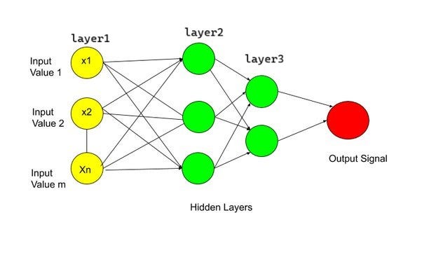
L1, L2 and L3 represent a sequence of three layers, where each layer is a stack of nodes added one on another. For mathematical modelling, let us vectorize all values including the input, the output and the intermediate weights. Keeping L2 as the reference layer, the input vector arises from output of layer L1. Whereas the output vector of L2 is fed as the input of L3. Similarly output of layer3 is treated as input for final output signal as shown in above diagram.
Backward-Propagation:
Now for the first iteration, we randomly choose weights and biases for the input value i.e., for the forward propagation.
And then we will calculate the loss function for the predicted value that is how much difference is there in between the observed & predicted value.
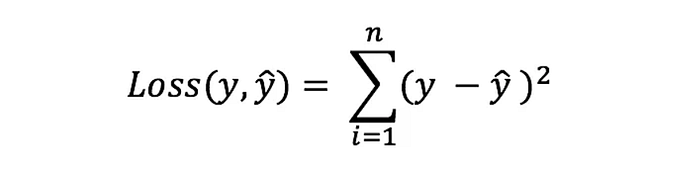
Here,
y => Observed Value
ŷ => Predicted Value
n => Total no of data-points

f( ) in the above equation is the activation function applied on the weighted sum of input vector. From the above equations, we can derive the notion that loss function clearly relates the total loss incurred by a model with a set of parameters, which are weights and biases.
Now, for minimizing the Loss Function we adjust weights and biases using an optimizer like Gradient-Descent and this process is called Back-Propagation.

Here, η is the learning rate, which is taken very very small value.
And Wx represents the respective weights of the following Input Value.
(L) in above equation represents Loss Function. Partial differentiation of Loss function with respect to respective weights is multiplied with learning rate.
In the backward propagation process, the model tries to update the parameters such that the overall predictions are more accurate. The forward propagation traverses from “left-to-right” or from the beginning of the network to the end, whereas the backward propagation moves from “right-to-left” or from the end of the network to the beginning.
